Lagrange Interpolation
Avoiding math by doing different math.
Or, how to avoid doing math...
...by doing different math!
Interpolation is a very common problem. You need to interpolate any time you have:
- A table of values, in larger increments than you'd like,
- A set of points on some unknown function,
- Known values some time apart, and you'd like to know what's in between.
Actually, these are all the same problem. Let's explore some solutions!
Bad Interpolation
There are a lot of techniques for interpolation. 90% of them are guaranteed to be bad, but I think it's a good idea to show why.
In real life, when I'm trying to interpolate something (maybe on the occasions I mess around with a cookbook) I try to "eyeball" it. For the amount of salt in a fractionally-scaled recipe, that's okay. (There is no such thing as too much salt. Fight me.) But for practical applications, we need to do better.
Back in The Old Days™, people had to consult log tables and/or slide rules for values of functions. This still happens today in astronomy, where orbital values come in tables called ephemerides, or almanacs, like these published by the United States Naval Observatory. If you want something between the given values, you need to interpolate.
Linear Interpolation
The simplest (formal) method is to fit the two points nearest your x-value to a line. If we know \(sin(x)\) at two points, say \(x = 0\) & \(x = 2\), then we might interpolate it like this:
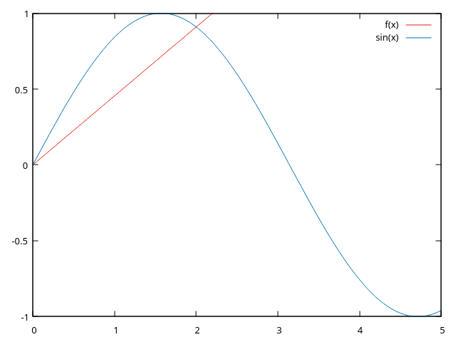
...which is objectively terrible. It could be better if we had a smaller increment than 0 to 2, but linear interpolation is inaccurate unless the thing it's interpolating is fairly linear itself. The upside is that it's easy to compute.
Smooth(er) Interpolation With Cosine
We can get a smoother curve by using weights on the interpolation function. We need something that produces a curve anywhere we like, so let's choose cosine. Now, given two points, we'll say: \[y_i \approx y_1 (1-\frac{1}{2}(1-cos(\pi \frac{x - x_1}{x_1-x_2})) + y_2 (\frac{1}{2}(1-cos(\pi \frac{x - x_1}{x_1-x_2}))\]
That's a mess. The \(\frac{x - x_1}{x_1-x_2}\) terms are our weight. When \(x\) is equal to \(x_1\), the term is zero, and all the weight is on \(y_2\). Conversely when \(x\) equals \(x_2\), the weight is one, and it's all on \(y_1\). Here's our visual example with the cosine interpolation added.
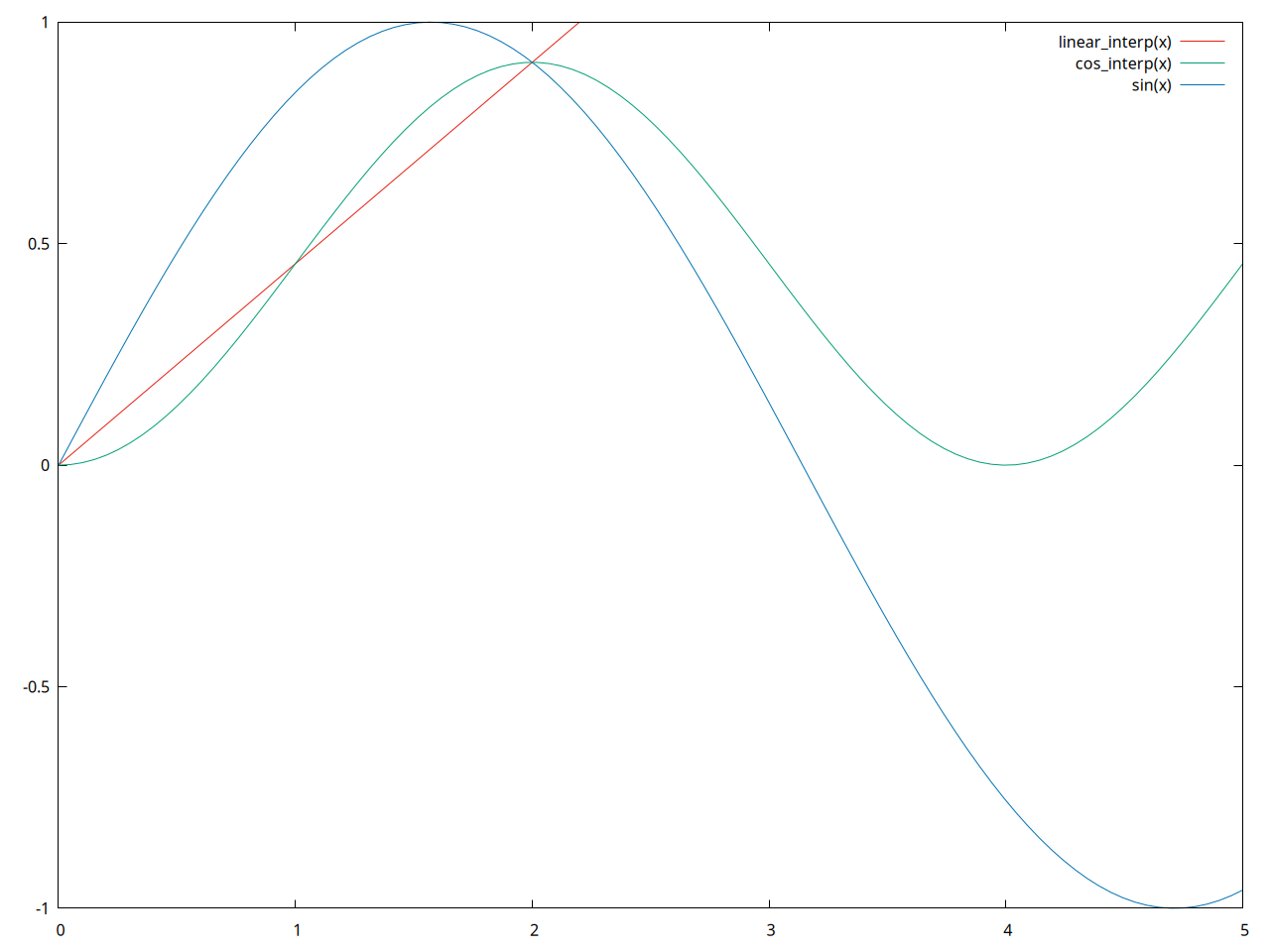
Notice that all this has done is smooth our linear function. It's still not precise. It would make a nice curve between multiple points, but let's try for something better.
Lagrange Polynomials and Lagrangian Interpolation
Let's be more ambitious. Say we have a set of \(n\) points (you decide how many) and we want to fit a polynomial to them. There will be many polynomials of degree \(> n\) that go through them, but only one of degree \(< n\). Usually, this polynomial's degree is \(n-1\). If the points happen to lie on a lower-degree polynomial, then the degree \(n-1\) polynomial's leading coefficients are zero.
Given our set of points \[(x_1, y_1), (x_2, y_2), ..., (x_i, y_i), ..., (x_n, y_n)\] the polynomial we want is this: \[y = \sum_{i=1}^n y_iL_i(x)\] where \(L_i(x)\) is the \(i\)th Lagrange polynomial, given by: \[L_i(x) = \prod_{j=1,j\ne i}^n\frac{x-x_j}{x_i-x_j}\]
In other words, the first Lagrange polynomial is: \[L_1(x) = \frac{(x-x_2)(x-x_3)...(x-x_n)}{(x_1-x_2)(x_1-x_3)...(x_1-x_n)}\]
We have a polynomial that goes through all the points, and it is also the polynomial of least degree that does so. (That's important for maximum accuracy.) The linked textbook walks through this topic in more detail, but I'll jump straight to my code.
To get a computer to do this for us, we'll first need to pull in our table of values, which is a vector of points in Computer-Science-ese, and evaluate the \(i\)th Lagrange polynomial at the \(x\)-value we want to interpolate, for all \(i\) in \([0,n]\). This just amounts to a couple of for-loops.
I used a janky iterator to exclude \(i\) in the internal loop. (Recall the provision \(j\ne i\) in our Lagrange polynomial definition.) I'm sure there's a better way to do this, but that's all I could come up with at the time...
fn lagrangian_interpolation(table: Table, xval: f64) -> f64 {
    let n = table.len();
    let mut sum = 0.0;

    for i in 0..n {
        if let Some(Point(x_i, y_i)) = table.pt_at(i) {
            // Evaluate the ith Lagrange poly'n. at xval and add it to sum.
            let mut product = 1.0;

            // Iterator grabs all but i.
            for j in (0..n)
                .enumerate()
                .filter(|&(pos, _)| (pos != i))
                .map(|(_, e)| e)
            {
                let x_j = table.pt_at(j).unwrap().0;
                product *= (xval - x_j) / (x_i - x_j);
            } // product is now the value of L_i(xval).

            sum += y_i * product;
        } else {
            break;
        }
    }

    sum
}
I set up my main function to print out a tab-separated list of points, and redirected this to a file. Then, I used gnuplot to plot these points in yellow, so we have a comparison of all our methods.
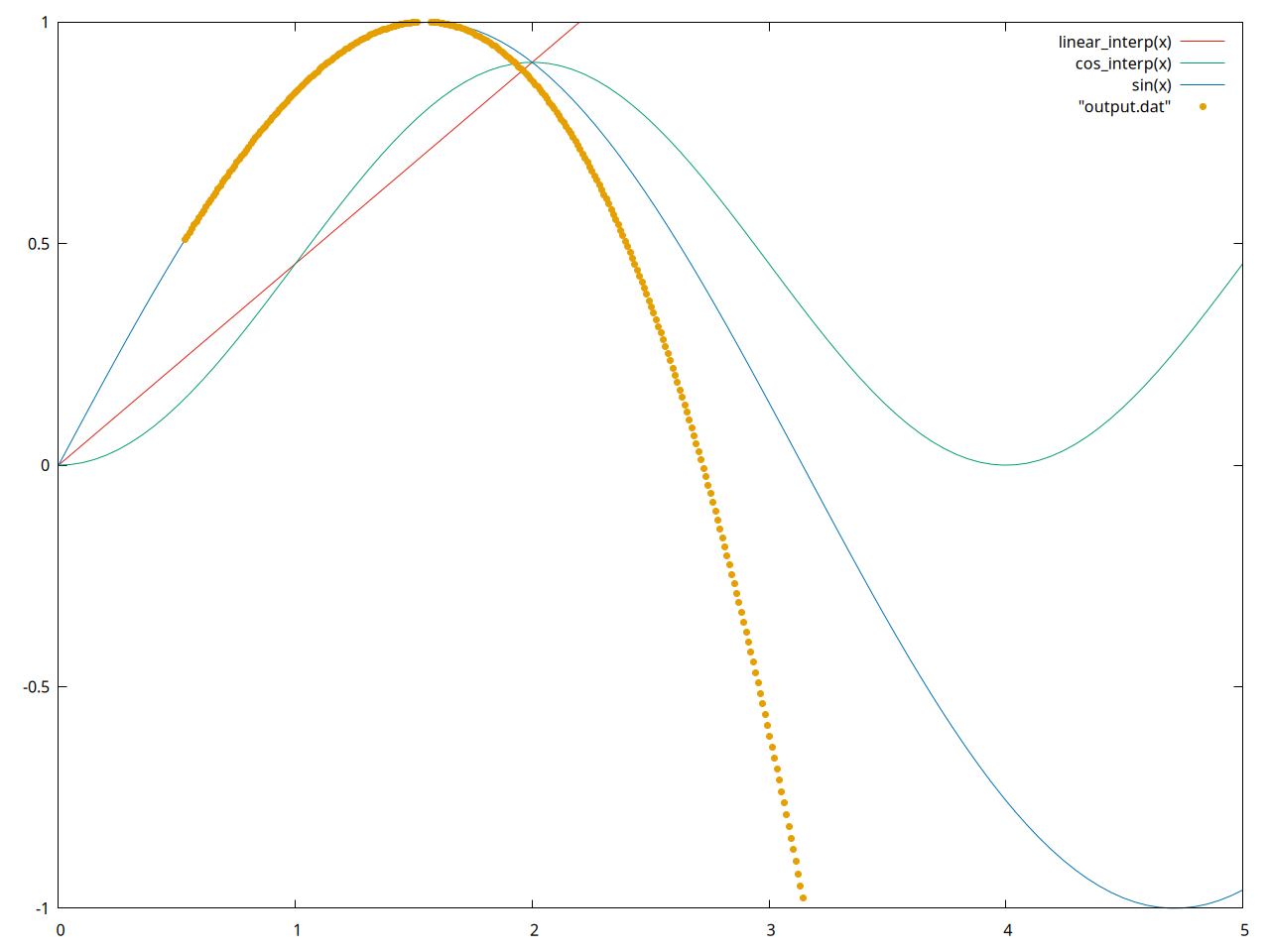
Notice that the yellow tracks the actual function in blue very well, until about 1.5 radians. I ran this test with a table of four values, and began interpolating points with roughly \(x = \frac{\pi}{6}\), in increments of \(0.01\), for 1000 iterations. It's extrapolating past my last tabulated value of \((1.5707963, 1.0)\), or \((\frac{\pi}{2}, 1)\), and doing an acceptable job for a little while.
The reader is welcome to try fixing the table so the interpolation is more accurate over the interval. All the Rust and gnuplot source code are in my repo here.
This technique is fairly fast, efficient, and is useful in Gaussian quadrature, as well as other modern applications. I hope you find it interesting, if not useful. Either way, let me know what you thought on GitHub, LinkedIn, or by email to ethan.barry@howdytx.technology!
References
Paul Bourke's classic 1999 post. His blog is pure gold; do yourself a favor and bookmark it.
Numerical Methods Guy, 2008:
This textbook on Celestial Mechanics, where I first learned about the Lagrange interpolation algorithm: