The Best Possible Quadrature Routine (Within Reason)
Gauss-Lobatto-Kronrod Quadratures
...in Rust, of course.
Originally all I wanted to do with numerical analysis was string together some functions and plot an ephemeris, given the right data. Planetary motions are fascinating, and I think it will be a really cool project. However, after reading the first chapter of the textbook Celestial Mechanics, where the author lists important numerical methods, I realized that numerical analysis by itself is something interesting.
In the last section of the first chapter he gives a list of programs or routines that are useful to him. One of those was using Gaussian quadrature to compute a definite integral. I already discussed the problem of quadrature in the post on Simpson's Rule, and I mentioned Gaussian quadrature specifically in the post on Lagrange interpolation. But, it's still worth revisiting the question of what quadrature means, before I share what I learned about Gaussian quadrature.
Computing Definite Integrals
In calculus we learn that a definite integral is actually the area beneath a curve. We approximate this with a sum of the areas of many small slices. In fact, the exact value is the number the sum approaches as the number of slices goes to infinity. This is called the Riemann sum approach, and essentially, it chops the integral up in nice rectangular bits. If we wanted to approximate an integral, one way would be to chop it up into lots of rectangles, and add their areas. If we want a closer approximation, then we just make finer slices.
This is certainly a fine method, but it would be a nightmare to compute by hand. Every slice needs its own function evaluation. Even in a computer, this can be slow. And, since we would be using rectangles to approximate a smooth function, this would still be inaccurate.
If, instead of using a flat-topped rectangle, we used a slope-topped trapezoid as our slice shape, we could make the slope line up with the function. That would mean our calculation would be more accurate, and would require fewer function evaluations. This is the trapezoid rule.
And, if we use a quadratic curve as the top of the slice, it can fit the function even more tightly still. That was Simpson's Rule, from my earlier post. In fact, there's a whole class of quadrature rules called Newton-Cotes formulas, which extend this idea, using higher-order polynomials to interpolate the points.
With these methods, we have one degree of freedom. We get to choose the weighting coefficients in equations like Simpson's Rule:
\[\int_a^b f(x)\,dx \approx \frac{1}{3}(f(a) + 4f(c) + f(b))\]
The big idea behind Gaussian quadrature is that it allows us to choose both the weights and the locations at which we evaluate \(f(x)\), giving us two degrees of freedom. With Newton-Cotes formulas, our accuracy increased at \(\mathcal{O}(n)\), as we added more slices. Now, we can converge to the result at \(\mathcal{O}(n^2)\), with the extra degree of freedom.
Let's examine the main idea.
Gaussian Quadrature
Simpson's Rule and the rest of the Newton-Cotes formulas essentially represent the integrand with polynomials. Gaussian quadrature lets us represent our integrand as a polynomial times a weight function. This is good, because some functions aren't nicely interpolated by polynomials. We can also evaluate at different points by applying weights to the evaluations.
This gives us the general Gaussian quadrature rule
\[\int_{-1}^1 W(x)f(x)\,dx \approx \sum_{1=0}^n w_if(x_i)\]
The polynomials we need to use are called Legendre polynomials. So, in our equation, \(n\) is the number of sample points, \(w_i\) are the weights, and \(x_i\) are the roots of the \(n\)th Legendre polynomial. The integral is given on the interval \([-1,1]\) because that is where Legendre polynomials have most of their useful properties, but we can scale up or down to any interval \([a,b]\).
We can compute the roots on the fly for any order \(n\), within reason. There is a technique called the Newton-Raphson method which finds roots of nonlinear functions. It takes a starting guess and iteratively improves it until the difference between the new value and the old one is within tolerance. It's a surprisingly simple technique.
\[x_{new} = x_{old} - \frac{f(x_{old})}{f'(x_{old})}\]
Now we just need the polynomials! There's a recurrence relation for them, so starting with the first two, we can build all the Legendre polynomials after that.
\[\begin{align}p_{-1}(x) &= 0\\ p_0(x) &= 1\\ p_{j+1}(x) &= (x-a_j)p_j(x) - b_jp_{j-1}(x),\quad j = 1,2,...,n\end{align}\]
We need a good guess to use Newton-Raphson. Usually the roots are closely approximated by \[r=\cos\left(\pi\frac{i + \frac{3}{4}}{n + \frac{1}{2}}\right)\quad i = 0,...,\frac{(n+1)}{2}\] where \(n\) is the order of the quadrature.
Once we have the weights \(w_i\), given by \[w_i = \frac{2}{(1-x_i^2)\left[p_n'(x_i)\right]^2}\] where \(p_n'\) is the derivative of the \(n\)th Legendre polynomial. Finally, we can mix all these numbers together in some code. But first, I want to show a result this algorithm gives.
Here's a test problem with the correct approximation to 9 decimal places: \[\int_0^1 \frac{ x^4 }{ \sqrt{ 2(1+x^2) }}\,dx \approx 0.108\,709\,465\,052\,586\,44\] The Rust code I wrote returns this value to nine decimal places with a 7-point Gauss-Legendre quadrature. That means the function only had to be evaluated seven times. I also used Simpson's Rule with seven evaluations, and it gave me an answer of 0.108 710, which is not bad.
Now, if I raise the Gaussian quadrature's order to eight, I get the answer 0.108 709 465 037, which is correct to 10 decimal places. If I raise the Simpson's Rule order to eight as well, I get 0.108 709 862, which is still only correct to six decimal places.
The code is below.
pub fn gaussian_quad<F>(f: F, a: f64, b: f64, n: u32) -> f64
where
    F: Fn(f64) -> f64,
{
    const NEWTON_PRECISION: f64 = 1.0e-10;
    let mut res = 0.0;
    // Scale the bounds of integration a and b to [-1, 1]
    // using the change of variables
    // x = st + c for t ∈ [-1, 1]
    // where
    // s = (b - a) / 2
    // and
    // c = (b + a) / 2.
    let s = (b - a) / 2.0;
    let c = (b + a) / 2.0;
    let m = (n + 1) / 2;
    let mut roots = vec![0.0; n as usize];
    let mut weights = vec![0.0; n as usize];
    for i in 0..m {
        // Approximate the ith root of this Legendre polynomial.
        let mut z = f64::cos(consts::PI * (i as f64 + 0.75) / (n as f64 + 0.5));
        let mut z1 = z - 1.0; // Ensure an initial difference.
        let mut p_prime = 0.0;
        while (z - z1).abs() > NEWTON_PRECISION {
            let mut p1 = 1.0;
            let mut p2 = 0.0;
            // Build the Legendre polynomial using the recurrence relation here...
            for j in 0..n {
                let p3 = p2;
                p2 = p1;
                p1 = ((2.0 * j as f64 + 1.0) * z * p2 - j as f64 * p3) / (j + 1) as f64;
            }
            // p1 is now the desired Legendre polynomial.
            // let p_prime be its derivative, computed by a known relation.
            p_prime = n as f64 * (z * p1 - p2) / (z * z - 1.0);
            z1 = z;
            z = z1 - p1 / p_prime; // Newton-Raphson method.
        }
        // z is now the ith root of the polynomial.
        roots[i as usize] = z;
        roots[(n - 1 - i) as usize] = -z;
        weights[i as usize] = 2.0 / ((1.0 - z * z) * p_prime * p_prime);
        weights[(n - 1 - i) as usize] = weights[i as usize];
    }

    for i in 0..n as usize {
        res += weights[i] * f(s * roots[i] + c);
    }
    res * s // Scale back to normal size.
}
Now, if we have a function that is well-behaved, this will work nicely. But if there's an irregularity in just one or two places, we have to raise the number of points just to cover those two subintervals. Wouldn't it be nice if we could somehow adapt to a problem like that, and only do more evaluations when we need them?
Adaptive Quadrature
Remember that the heart of numerical integration is chopping area into smaller pieces. If there's an interval where the function goes crazy, and one where it's smooth, then let's not worry about the smooth interval too much, and focus on the crazy one. How do we measure "craziness?" The general method is to evaluate the integral on the interval twice—once at low precision, then again at high precision—which gives us a difference. If that difference is within a tolerance, then we leave it alone. If not, we split the interval and repeat the process.
You might think that this will cost us a lot of function evaluations. It will take more, but maybe we can minimize the number needed. And an adaptive routine is already saving us evaluations in comparison to just globally increasing evaluations to boost accuracy, like with Simpson's Rule.
With Gaussian quadrature, a low-precision rule will not have the same \(x\)-coordinates as a high-precision one. That means we can't reuse any of those function values. What we're looking for is a nested quadrature, which "nests" a higher-order quadrature inside a lower-order one. There are two options, Clenshaw-Curtis, and Gauss-Kronrod. Both were invented around 1960; the first by two Western (British, I think) mathematicians, and the second by a Soviet mathematician, Aleksandr Semyonovich Kronrod.
This particular algorithm, from the paper "Adaptive Quadrature—Revisited" by W. Gander and W. Gautschi, is an example of Gauss-Lobatto-Kronrod quadrature. Kronrod's extension of Gaussian quadrature allows us to reuse function evaluations for higher precision, and the "Lobatto" part means we use the endpoints as well.
A Kronrod Rule uses \(2n+1\) points, where \(n\) is the number of points for the Gaussian quadrature. This makes the Kronrod Rule exact for a polynomial up to degree \(3n+1\). The extra \(x\)-values (abscissas) are nowadays calculated with some linear algebra tricks, as described in the paper. They can also be found by solving non-linear equations with Newton's Method, but because either one would be expensive, we'll use tabulated values.
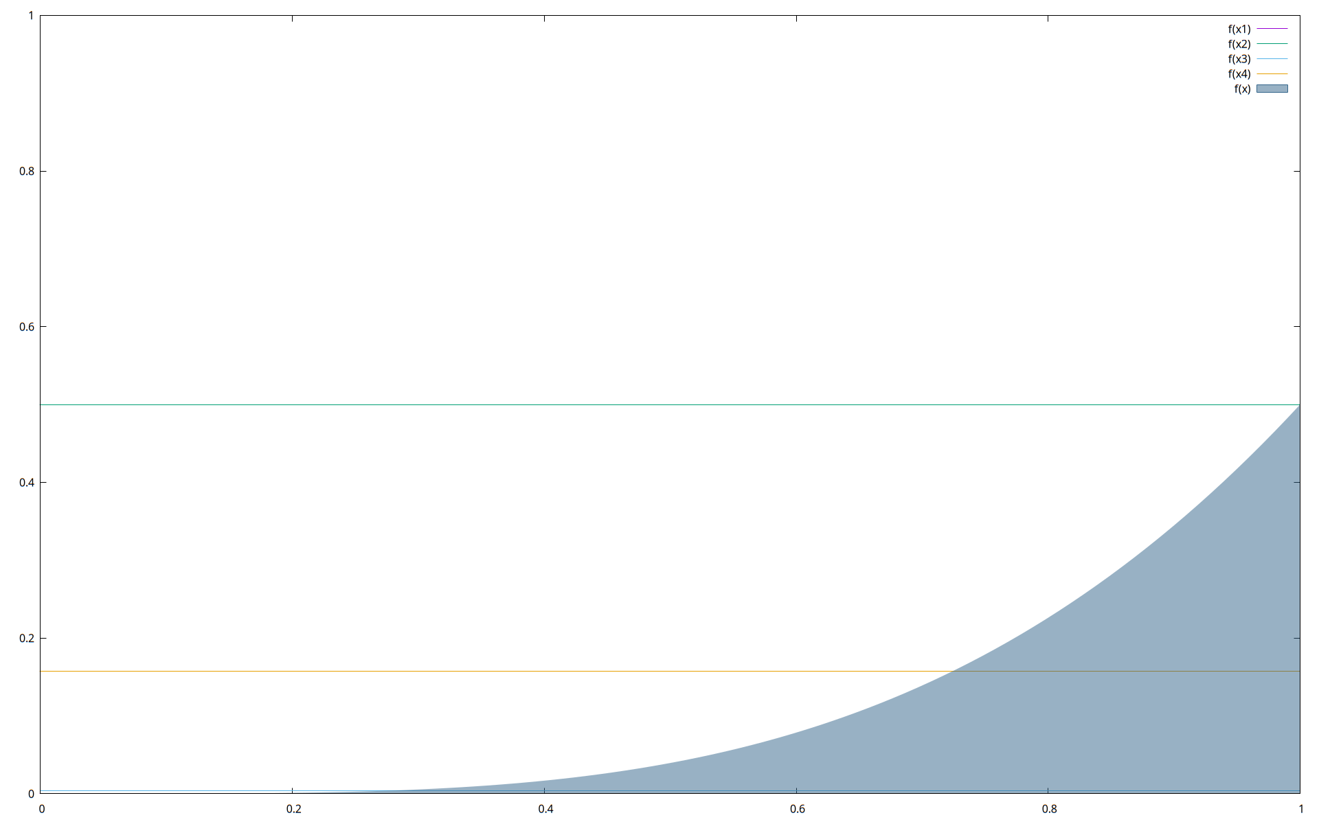
As an example of what Gaussian quadrature and the Kronrod extension are really doing, I produced a little graphic with gnuplot. Here is a 4-point Gauss-Lobatto quadrature of our example \(\int_0^1 \frac{ x^4 }{ \sqrt{ 2(1+x^2) }}\,dx\). The lines pass through the \(y\)-values of the Gaussian abscissas, so the abscissas lie below the intersection of the line and the curve. The Kronrod abscissas would occur somewhere between the Gaussian ones.
The function I created has a pretty simple interface. I didn't include controls on how many iterations to allow, or what precision to calculate the integral to. It simply computes until the answer is stable to within machine precision.
pub fn gaussian_kronrod_quad<F>(func: F, a: f64, b: f64) -> f64
where
    F: Fn(f64) -> f64,
{
/* SNIP; CODE BELOW */
}
This has given very good results on the integrals I've tested. For example, on our problem from earlier, \[\int_0^1 \frac{ x^4 }{ \sqrt{ 2(1+x^2) }}\,dx \approx 0.108\,709\,465\,052\,586\,44\] I get the answer to the ~17 digits allowed by a double precision float f64.
The basic steps are:
- Evaluate a 4-point Gauss-Lobatto quadrature on the scaled interval.
- Evaluate a 7-point Kronrod extension using the 4-point values.
- Evaluate a general estimate for the entire integral with a 13-point Kronrod extension using stored values from the previous two.
- If the 4- and 7-point values differ by more than machine precision, split the interval into six parts, and perform the same 4- & 7-point procedure on those. Add their results.
This is a very good quadrature method, comparable to Julia's QuadGK.jl package, or some tools from other dedicated systems, like GNU OCTAVE and MATLAB. In fact, in the paper linked above, the authors show that it was actually an improvement over the quadatures available at the time in MATLAB, and the NAG and IMSL libraries.
Conclusion
The speed and type safety of Rust make it a very attractive option for scientific computing, but so far, it hasn't made much headway against more established languages like FORTRAN, Python, and Julia. The numerical analysis and linear algebra packages in Rust are improving, but they're often less-complete than counterparts elsewhere.
I think the killer application of Rust in this space might be concurrency. Rust makes parallelization much more achievable. Rust's SIMD wrappers are nicer than most languages' equivalents as well, so parallelizing and vectorizing sci-comp workloads is a unique benefit Rust can offer. I'm excited to see what happens in this space.
/// An adaptive 4-point Gauss-Lobatto quadrature routine.
/// Kronrod's Rule is used to reduce the computations needed,
/// while using 7- & 13-point Kronrod quadratures for error checking.
///
/// ## Inputs
/// - f: The integrand (must be integrable on \[a,b\])
/// - a: The lower bound of integration.
/// - b: The upper bound of integration.
///
/// NOTE: The algorithm assumes a < b.
/// ## Outputs
/// An `f64` value containing the definite integral calculated to machine precision.
/// ## Examples
/// ```rust
/// use symmetria::quadrature::gaussian_kronrod_quad;
/// use std::f64::consts;
/// let f = |x: f64| x.cos();
/// let val = gaussian_kronrod_quad(f, 0.0, (consts::PI / 2.0));
/// assert!((1.0 - val).abs() < 1.0e-17);
/// ```
pub fn gaussian_kronrod_quad<F>(func: F, a: f64, b: f64) -> f64
where
    F: Fn(f64) -> f64,
{
    // This algorithm was adopted from the paper
    // "Adaptive Quadrature --- Revisited" by Walter Gander and Walter Gautschi.
    // published in BIT Numerical Mathematics, vol. 40, No. 1, pp. 84-101.

    // Scale the bounds of integration a and b to [-1, 1].
    // This converts
    // \int_a^b f(x)dx to \int_{-1}^1 f(sx + c)sdx
    // using the change of variables
    // x = scale * t + coscale for t ∈ [-1, 1]
    // where
    // scale = (b - a) / 2
    // and
    // coscale = (b + a) / 2.
    let scale = (b - a) / 2.0;
    let coscale = (b + a) / 2.0;
    // Now, f must always be evaluated at scale * x + coscale, not simply x, and the answer multiplied by scale.

    let gl4_weights = [1.0 / 6.0, 5.0 / 6.0];
    let gl4_fnevals = [
        func(scale * -1.0 + coscale),
        func(scale * 1.0 + coscale),
        func(scale * -1.0 / 5.0_f64.sqrt() + coscale),
        func(scale * 1.0 / 5.0_f64.sqrt() + coscale),
    ];
    // Next, use the 4-point Gauss-Lobatto quadrature given by
    // \int_{-1}^1 f(x)dx ≈ \frac{1}{6}[f(-1) + f(1)]
    //                      + \frac{5}{6}[f(-\frac{1}{\sqrt{5}}) + f(\frac{1}{\sqrt{5}})]
    let gl4 = gl4_weights[0] * ((gl4_fnevals[0] + gl4_fnevals[1]) * scale)
        + gl4_weights[1] * ((gl4_fnevals[2] + gl4_fnevals[3]) * scale);

    let kron7_fnevals = [
        func(scale * -((2. / 3.0_f64).sqrt()) + coscale),
        func(scale * (2. / 3.0_f64).sqrt() + coscale),
        func(coscale), // scale * 0.0 is 0.
    ];
    // Then we compare this to its 7-point Kronrod extension, given by
    // \int_{-1}^1 f(x)dx ≈ \frac{11}{210}[f(-1) + f(1)]
    //                      + \frac{72}{245}[f(-\sqrt{\frac{2}{3}}) + f(\sqrt{\frac{2}{3}})]
    //                      + \frac{125}{294}[f(-\frac{1}{\sqrt{5}}) + f(\frac{1}{\sqrt{5}})]
    //                      + \frac{16}{35}[f(0)]
    let kron7 = (11. / 210.) * ((gl4_fnevals[0] + gl4_fnevals[1]) * scale)
        + (72. / 245.) * ((kron7_fnevals[0] + kron7_fnevals[1]) * scale)
        + (125. / 294.) * ((gl4_fnevals[2] + gl4_fnevals[3]) * scale)
        + (16. / 35.) * (kron7_fnevals[2] * scale);

    // Finally, we compare all of them to the 13-point Kronrod extension, given by
    // \int_{-1}^1 f(x)dx ≈ A * [f(-1) + f(1)]
    //                      + B * [f(-x_1) + f(x_1)]
    //                      + C * [f(-\sqrt{\frac{2}{3}}) + f(\sqrt{\frac{2}{3}})]
    //                      + D * [f(-x_2) + f(x_2)]
    //                      + E * [f(-\frac{1}{\sqrt{5}}) + f(\frac{1}{\sqrt{5}})]
    //                      + F * [f(-x_3) + f(x_3)]
    //                      + G * [f(0)]
    // where
    // A = .015827191973480183087169986733305510591,
    // B = .094273840218850045531282505077108171960,
    // C = .15507198733658539625363597980210298680,
    // D = .18882157396018245442000533937297167125,
    // E = .19977340522685852679206802206648840246,
    // F = .22492646533333952701601768799639508076,
    // G = .24261107190140773379964095790325635233,
    // and
    // x_1 = .94288241569547971905635175843185720232,
    // x_2 = .64185334234578130578123554132903188354,
    // x_3 = .23638319966214988028222377349205292599.
    let a_weight = 0.015_827_191_973_480_183;
    let b_weight = 0.094_273_840_218_850_05;
    let c = 0.155_071_987_336_585_4;
    let d = 0.188_821_573_960_182_45;
    let e = 0.199_773_405_226_858_52;
    let f = 0.224_926_465_333_339_51;
    let g = 0.242_611_071_901_407_74;

    let x_1 = 0.942_882_415_695_479_7;
    let x_2 = 0.641_853_342_345_781_3;
    let x_3 = 0.236_383_199_662_149_88;

    let kron13 = a_weight * (gl4_fnevals[0] + gl4_fnevals[1]) * scale
        + b_weight * (func(scale * -x_1 + coscale) + func(scale * x_1 + coscale)) * scale
        + c * (kron7_fnevals[0] + kron7_fnevals[1]) * scale
        + d * (func(scale * -x_2 + coscale) + func(scale * x_2 + coscale)) * scale
        + e * (gl4_fnevals[2] + gl4_fnevals[3]) * scale
        + f * (func(scale * -x_3 + coscale) + func(scale * x_3 + coscale)) * scale
        + g * kron7_fnevals[2] * scale;

    let x = vec![a, b];
    let y = batch_eval(&func, &x);

    gkquad_recursive(&func, a, b, y[0], y[1], kron13)
}

/// A helper function for gaussian_kronrod_quad().
fn gkquad_recursive<F>(f: &F, a: f64, b: f64, fa: f64, fb: f64, iest: f64) -> f64
where
    F: Fn(f64) -> f64,
{
    let h = (b - a) / 2.0;
    let m = (a + b) / 2.0;
    let alpha = f64::sqrt(2.0 / 3.0);
    let beta = 1.0 / f64::sqrt(5.0);

    // Our new evaluation points...
    let mll = m - alpha * h;
    let ml = m - beta * h;
    let mr = m + beta * h;
    let mrr = m + alpha * h;
    let x = vec![mll, ml, m, mr, mrr];
    let y = batch_eval(&f, &x);

    let fmll = y[0];
    let fml = y[1];
    let fm = y[2];
    let fmr = y[3];
    let fmrr = y[4];

    let i2 = (h / 6.0) * (fa + fb + 5.0 * (fml + fmr));
    let i1 =
        (h / 1470.) * (77. * (fa + fb) + 432. * (fmll + fmrr) + 625. * (fml + fmr) + 672. * fm);

    if iest + (i1 - i2) == iest || mll <= a || b <= mrr {
        if m <= a || b <= m {
            // At this point, we have exhausted the machine's precision.
            // We should handle this somehow...
        }
        i1
    } else {
        // Sum of the integrals on the ranges [a, mll], [mll, ml], [ml, m], [m, mr], [mr, mrr], [mrr, b];
        gkquad_recursive(f, a, mll, fa, fmll, iest)
            + gkquad_recursive(f, mll, ml, fmll, fml, iest)
            + gkquad_recursive(f, ml, m, fml, fm, iest)
            + gkquad_recursive(f, m, mr, fm, fmr, iest)
            + gkquad_recursive(f, mr, mrr, fmr, fmrr, iest)
            + gkquad_recursive(f, mrr, b, fmrr, fb, iest)
    }
}
NOTE: The function doesn't initially check whether it ought to evaluate recursively or not, but a simple if-else statement should catch that.